In this post, we will look at the example of TwinAPI- TemperatureCube, which makes it possible to mesh the cube geometry, which is one of the simple geometries frequently used in engineering problems, and to make a solution by giving different boundary conditions. In the example, firstly, we see that the modules named Mesher and Solver are imported.  

Mesher used to create geometry and mesh, and Solver used to create solutions in the created geometry are the two main modules of TwinAPI. Geometries such as cube, I beam, L beam, and mesh elements which are frequently used in engineering problems in the Mesher module, have been pre-created for you. In Solver module, formulas and programs used in heat transfer calculations are brought together for users. At TwinAPI, all users have to do is to use these modules and the appropriate functions, and to give the parameters of the system they want to create to the system in a few lines.  

Since the Analysis function of the Solver module will be used frequently while setting up our system, we create a new variable called BarTemp that calls the Analysis function. We choose our solver using the SetSolver command in BarTemp. In this example, corefem, which is Simularge's own solver, is used. You can also choose CalculiX as a solver. It will be sufficient to use the Unit Cube function of the Mesher module to create the unit cube in the mesh creation section. We specify how many elements we want to create a mesh in the Unit Cube function. In this example, we see that a 5-element body with a tetrahedral mesh structure named box1 has been created. This body will then be used in the boundary conditions section. In the Material section, we specify which type of material we want our unit cube to consist of. According to the material type mentioned here, the material properties will be adjusted for us from the material library in the background. Currently, there are options such as aluminum (AL), steel (STEEL). In the future, updates will be made in the material library.

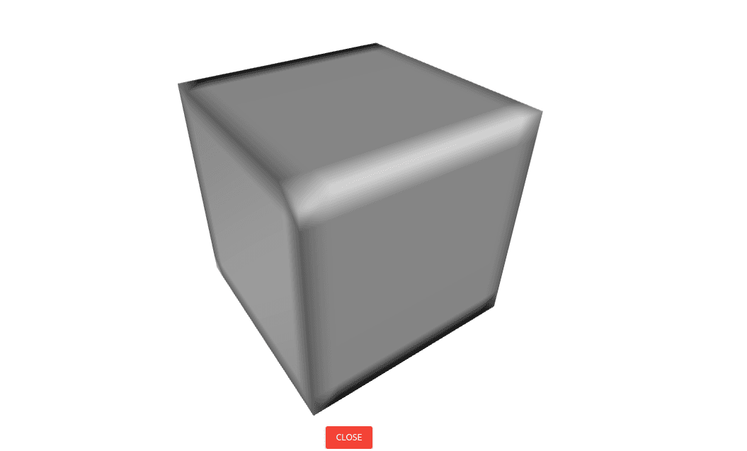
We add the specified mesh and the material to the system as a part with the BarTemp.AddPart function, and then use the BarTemp.Assemble function to create a mesh that conforms to the specified features. After this step, by pressing the Run button and then the Preview button, we can view the unit cube geometry we have created as shown in the figure below.

Now that we have completed the meshing part, we can move on to the necessary adjustments for the solution. With Solver.CreateStep, we create a step and make all our adjustments through this step. With the Time function, we enter the steady state/ transient and the start, end times and time step of the solution.With the AddBC function, we specify which type of boundary condition we will give to which surface of the body and the size of these boundary conditions. And then we create this solution and run it with the Solve function. Finally,we can use the result function to print the solution results for a specific point.

After completing all the settings for the system we want to solve, we can now press the Run button and see the solution result printed in the Output section and visually in the Graph section. In this example,the steady state temperature of the specified (0, 0, 0) point has been obtained as output as shown in the figure below.

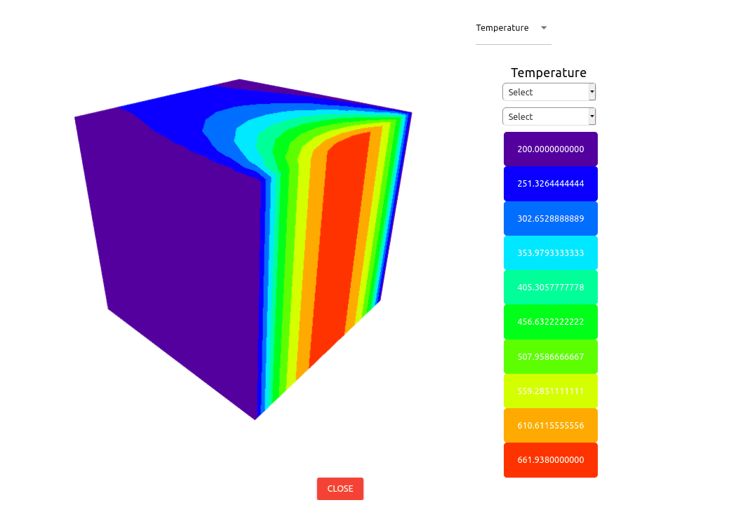
You can click the Result button to view the temperature distribution on the whole geometry as shown in the figure below.

In this example, since a steady state analysis is performed, we can seethe temperature of the point we are interested in when it reaches the steady state. You can also see a time-dependent solution in the Temperature Cube Transient example. Please feel free to review the examples, and share your comments and questions with us. More to come, follow our blog page and visit https://www.twinapi.com and register for free today!